Lab 10

Continuing Seaborn

We’ll finish up the seaborn material from last lab

Multidimensional Scaling (MDS)

Note: This is based off of Prof Tony Jebara’s lecture notes for COMS 6772 at Columbia in Spring 2015.

Say we have a series of points \(x_1,\ldots,x_n \in R^d\), where \(d\) is large, and we want to learn a representation of these data in \(R^k\) with \(k << d\) (as we do in Project 2 to visualize Presidents and speeches).

How can we do this?

Idea: Find a representation that preserves pairwise distances between the data. In general we don’t need to just consider distances, but can widen our scope to dissimilarities. A Dissimilarity is a function \(d:R^d \times R^d \to R\) such that for all \(x,y \in R^d\).

• \(d(x,y) \geq 0\)
• \(d(x,x) = 0\)
• \(d(x,y) = d(y,x)\)

Two examples which are both distances and dissimilarities are the usual Euclidean distance between vectors and the Jensen-Shannon distance for distributions.

For our data \(x_1,\ldots,x_n\), we can construct the matrix of pairwise dissimilarities as

\[\Delta_{ij} = d(x_i, x_j)\]

Now we can formalize the problem a bit more. Given data \(x_1,\ldots,x_n \in R^d\) with dissimilarity matrix \(\Delta\), can we find a representation \(y_1,\ldots,y_n \in R^k\) with dissimilarity matrix \(D\) such that \(D\) is “close” to \(\Delta\).

How do we define “close”? Scikit learn uses Stress:

\[Stress(y_1,\ldots,y_n) = \sum_{ij} (D_{ij} - \Delta_{ij})^2\]

To find a lower-dimensional representation we then find \(y_1,\ldots,y_n \in R^k\) to minimize the stress.

Let’s look at an example with the NFL trends data from Lab 9.

import pandas as pd
import numpy as np
import matplotlib.pyplot as plt
import seaborn as sns
%matplotlib inline
sns.set_style("whitegrid")

# load the data
nfl_trends = pd.read_csv("data/fivethirtyeight-nfl-google.csv", header=1)
nfl_trends.head()
# convert percent strings into floats
numeric_data = (nfl_trends.iloc[:,1:]
                .replace("%", "",regex=True)
                .astype(float))
numeric_data["DMA"] = nfl_trends["DMA"]
nfl_trends = numeric_data

We’ll normalize the search interest for each league in each market (they’re actually close to adding up to 100 except for rounding errors).

# get the search interest for each league, normalizes
interests  = nfl_trends.iloc[:,:-2].values
interests = interests / interests.sum(1, keepdims=True)

Now we can compute the Jensen-Shannon distance between all of the markets and get a distance matrix.

from scipy.stats import entropy

def JSdiv(p, q):
    """Jensen-Shannon divergence."""
    m = (p + q) / 2
    return (entropy(p, m, base=2.0) + entropy(q, m, base=2.0)) / 2

# initialize the distance matrix
n = interests.shape[0]
dist = np.zeros((n,n))
# compute JS distance for all pairs
for i in range(n):
    for j in range(n):
        dist[i,j] = JSdiv(interests[i,:], interests[j,:])

And use MDS to find a lower dimensional representation

from sklearn import manifold

# intiialize
MDS =  manifold.MDS(dissimilarity="precomputed")
# transform to lower dimensional representation with JS distance
lower = MDS.fit_transform(dist)

# intiialize
MDS =  manifold.MDS()
# transform to lower dimensional representation with Euclidean distance
lower_naive = MDS.fit_transform(interests)

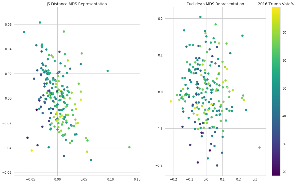
# put into a dataframe and plot
lower_df = pd.DataFrame({"x_JS":lower[:,0], "y_JS":lower[:,1],
                         "x_naive":lower_naive[:,0], "y_naive": lower_naive[:,1],
                         "DMA":nfl_trends["DMA"],
                        "Trump 2016 Vote%":nfl_trends["Trump 2016 Vote%"]})

fig, (ax1, ax2) = plt.subplots(1, 2, figsize=(16,10))
s = ax1.scatter(lower_df["x_JS"], lower_df["y_JS"], c=lower_df["Trump 2016 Vote%"],
           cmap=plt.get_cmap("viridis"))
s = ax2.scatter(lower_df["x_naive"], lower_df["y_naive"], c=lower_df["Trump 2016 Vote%"],
           cmap=plt.get_cmap("viridis"))

ax1.set_title("JS Distance MDS Representation")
ax2.set_title("Euclidean MDS Representation")

cbar = fig.colorbar(s)
cbar.ax.set_title("2016 Trump Vote%");

/home/ebenmichael/anaconda3/lib/python3.6/site-packages/matplotlib/font_manager.py:1297: UserWarning: findfont: Font family ['sans-serif'] not found. Falling back to DejaVu Sans
  (prop.get_family(), self.defaultFamily[fontext]))