Exploratory analysis #3: investor portfolio correlations
Do investors cluster together? In other words, if a company can get a certain investor, are there others the company is likely to get as well? In this notebook we consider the correlation among investors using multidimensional scaling.
In [1]:
from modules import *
In [2]:
%matplotlib inline
import matplotlib.pyplot as plt
import seaborn as sns
import numpy as np
import pandas as pd
from collections import Counter

plt.style.use('seaborn-dark')
plt.rcParams['figure.figsize'] = (10, 6)
In [3]:
# connect to mysql db, read cb_investments, cb_objects, and cb_funds as dataframes, disconnect
conn = dbConnect()
inv = dbTableToDataFrame(conn, 'cb_investments')
objs = dbTableToDataFrame(conn, 'cb_objects')
fund = dbTableToDataFrame(conn, 'cb_funds')
conn.close()
Look at the dataframes we’ve read in.
In [4]:
inv.head()
Out[4]:
| created_at | funded_object_id | funding_round_id | id | investor_object_id | updated_at | |
|---|---|---|---|---|---|---|
| 0 | 2007-07-04 04:52:57 | c:4 | 1 | 1 | f:1 | 2008-02-27 23:14:29 |
| 1 | 2007-07-04 04:52:57 | c:4 | 1 | 2 | f:2 | 2008-02-27 23:14:29 |
| 2 | 2007-05-27 06:09:10 | c:5 | 3 | 3 | f:4 | 2013-06-28 20:07:23 |
| 3 | 2007-05-27 06:09:36 | c:5 | 4 | 4 | f:1 | 2013-06-28 20:07:24 |
| 4 | 2007-05-27 06:09:36 | c:5 | 4 | 5 | f:5 | 2013-06-28 20:07:24 |
In [5]:
fund.head()
Out[5]:
| created_at | fund_id | funded_at | id | name | object_id | raised_amount | raised_currency_code | source_description | source_url | updated_at | |
|---|---|---|---|---|---|---|---|---|---|---|---|
| 0 | 2008-12-17 03:07:16 | 1 | 2008-12-16 | 1 | Second Fund | f:371 | 300000000 | USD | peHub | http://www.pehub.com/26194/dfj-dragon-raising-... | 2008-12-17 03:07:16 |
| 1 | 2008-12-18 22:04:42 | 4 | 2008-12-17 | 4 | Sequoia Israel Fourth Fund | f:17 | 200750000 | USD | Sequoia Israel Raises Fourth Fund | http://www.pehub.com/26725/sequoia-israel-rais... | 2008-12-18 22:04:42 |
| 2 | 2008-12-31 09:47:51 | 5 | 2008-08-11 | 5 | Tenth fund | f:951 | 650000000 | USD | Venture Beat | http://venturebeat.com/2008/08/11/interwest-cl... | 2008-12-31 09:47:51 |
| 3 | 2009-01-01 18:13:44 | 6 | None | 6 | New funds acquire | f:192 | 625000000 | USD | U.S. Venture Partners raises $625M fund for ne... | http://venturebeat.com/2008/07/28/us-venture-p... | 2009-01-01 18:16:27 |
| 4 | 2009-01-03 09:51:58 | 7 | 2008-05-20 | 7 | Third fund | f:519 | 200000000 | USD | Venture Beat | http://venturebeat.com/2008/05/20/disneys-stea... | 2013-09-03 16:34:54 |
In [6]:
objs.head()
Out[6]:
| category_code | city | closed_at | country_code | created_at | created_by | description | domain | entity_id | entity_type | ... | parent_id | permalink | region | relationships | short_description | state_code | status | tag_list | twitter_username | updated_at | |
|---|---|---|---|---|---|---|---|---|---|---|---|---|---|---|---|---|---|---|---|---|---|
| 0 | web | Seattle | None | USA | 2007-05-25 06:51:27 | initial-importer | Technology Platform Company | wetpaint-inc.com | 1 | Company | ... | None | /company/wetpaint | Seattle | 17.0 | None | WA | operating | wiki, seattle, elowitz, media-industry, media-... | BachelrWetpaint | 2013-04-13 03:29:00 |
| 1 | games_video | Culver City | None | USA | 2007-05-31 21:11:51 | initial-importer | None | flektor.com | 10 | Company | ... | None | /company/flektor | Los Angeles | 6.0 | None | CA | acquired | flektor, photo, video | None | 2008-05-23 23:23:14 |
| 2 | games_video | San Mateo | None | USA | 2007-08-06 23:52:45 | initial-importer | there.com | 100 | Company | ... | None | /company/there | SF Bay | 12.0 | None | CA | acquired | virtualworld, there, teens | None | 2013-11-04 02:09:48 | |
| 3 | network_hosting | None | None | None | 2008-08-24 16:51:57 | None | None | mywebbo.com | 10000 | Company | ... | None | /company/mywebbo | unknown | NaN | None | None | operating | social-network, new, website, web, friends, ch... | None | 2008-09-06 14:19:18 |
| 4 | games_video | None | None | None | 2008-08-24 17:10:34 | None | None | themoviestreamer.com | 10001 | Company | ... | None | /company/the-movie-streamer | unknown | NaN | None | None | operating | watch, full-length, moives, online, for, free,... | None | 2008-09-06 14:19:18 |
5 rows × 40 columns
Merge all three dataframes into one dataframe called allData to be used in all subsequent analysis in this workbook.
In [7]:
a = pd.merge(inv, objs, left_on = 'funded_object_id', right_on='id', suffixes=['_i', '_o'])
In [8]:
allData = pd.merge(a, fund, left_on = 'investor_object_id', right_on='object_id', suffixes=['_a', '_f'])
In [9]:
allData.head()
Out[9]:
| created_at_i | funded_object_id | funding_round_id | id_i | investor_object_id | updated_at_i | category_code | city | closed_at | country_code | ... | fund_id | funded_at | id | name_f | object_id | raised_amount | raised_currency_code | source_description | source_url | updated_at | |
|---|---|---|---|---|---|---|---|---|---|---|---|---|---|---|---|---|---|---|---|---|---|
| 0 | 2007-07-04 04:52:57 | c:4 | 1 | 1 | f:1 | 2008-02-27 23:14:29 | news | San Francisco | None | USA | ... | 99 | 2013-09-10 | 99 | Greylock Fund XIV | f:1 | 1000000000 | USD | Greylock Partners raises $1 billion for new ve... | http://www.reuters.com/article/2013/09/10/us-v... | 2013-09-10 19:05:00 |
| 1 | 2007-07-04 04:52:57 | c:4 | 1 | 1 | f:1 | 2008-02-27 23:14:29 | news | San Francisco | None | USA | ... | 420 | 2011-03-01 | 420 | Greylock Fund XIII | f:1 | 1000000000 | USD | Greylock: $1 billion more and new fund for “wi... | http://venturebeat.com/2011/03/01/greylock-1-b... | 2013-09-10 18:53:02 |
| 2 | 2007-07-04 04:52:57 | c:4 | 1 | 1 | f:1 | 2008-02-27 23:14:29 | news | San Francisco | None | USA | ... | 1446 | 2005-11-14 | 1446 | Greylock Fund XII | f:1 | 500000000 | USD | Greylock locks up 12th fund at $500M | http://www.bizjournals.com/boston/blog/mass-hi... | 2013-09-10 19:05:00 |
| 3 | 2007-07-04 04:56:09 | c:4 | 85 | 144 | f:1 | 2008-02-27 23:14:29 | news | San Francisco | None | USA | ... | 99 | 2013-09-10 | 99 | Greylock Fund XIV | f:1 | 1000000000 | USD | Greylock Partners raises $1 billion for new ve... | http://www.reuters.com/article/2013/09/10/us-v... | 2013-09-10 19:05:00 |
| 4 | 2007-07-04 04:56:09 | c:4 | 85 | 144 | f:1 | 2008-02-27 23:14:29 | news | San Francisco | None | USA | ... | 420 | 2011-03-01 | 420 | Greylock Fund XIII | f:1 | 1000000000 | USD | Greylock: $1 billion more and new fund for “wi... | http://venturebeat.com/2011/03/01/greylock-1-b... | 2013-09-10 18:53:02 |
5 rows × 57 columns
In [10]:
allData.shape
Out[10]:
(71811, 57)
In [11]:
allData.columns
Out[11]:
Index(['created_at_i', 'funded_object_id', 'funding_round_id', 'id_i',
       'investor_object_id', 'updated_at_i', 'category_code', 'city',
       'closed_at', 'country_code', 'created_at_o', 'created_by',
       'description', 'domain', 'entity_id', 'entity_type', 'first_funding_at',
       'first_investment_at', 'first_milestone_at', 'founded_at',
       'funding_rounds', 'funding_total_usd', 'homepage_url', 'id_o',
       'invested_companies', 'investment_rounds', 'last_funding_at',
       'last_investment_at', 'last_milestone_at', 'logo_height', 'logo_url',
       'logo_width', 'milestones', 'name_a', 'normalized_name', 'overview',
       'parent_id', 'permalink', 'region', 'relationships',
       'short_description', 'state_code', 'status', 'tag_list',
       'twitter_username', 'updated_at_o', 'created_at', 'fund_id',
       'funded_at', 'id', 'name_f', 'object_id', 'raised_amount',
       'raised_currency_code', 'source_description', 'source_url',
       'updated_at'],
      dtype='object')
Now create company matrix for entire set of investors. In company matrix, the index denotes the company and the column labels denote the investor. The matrix entry counts the number of occurences of each company in the investor portfolio.
In [12]:
# create dictionary with list of companies funded for each investor
investors = pd.unique(allData.investor_object_id).tolist()
i = 0
f = [None] * len(investors)
for investor in investors:
    allData_investor = allData[allData.investor_object_id == investor]
    f[i] = allData_investor.funded_object_id
    i = i+1
d = dict(zip(investors, f))
In [13]:
#companies is a list of all companies
companies = pd.unique(allData.funded_object_id).tolist()

# initialize empty dataframe with rownames as the unique companies
cmat = pd.DataFrame([], index = companies)

# for each investor, have list of companies and store as investors

# need a counter for column names
i = 0

# loop through the investors
for investor, c in d.items():
    #create column of data frame
    column = company_vector(c, companies)
    #create index name
    index = str(i)
    #add column
    cmat[index] = column
    #update index
    i = i + 1

cmat[500:510]
Out[13]:
| 0 | 1 | 2 | 3 | 4 | 5 | 6 | 7 | 8 | 9 | ... | 749 | 750 | 751 | 752 | 753 | 754 | 755 | 756 | 757 | 758 | |
|---|---|---|---|---|---|---|---|---|---|---|---|---|---|---|---|---|---|---|---|---|---|
| c:78697 | 0 | 0 | 0 | 6 | 0 | 0 | 0 | 0 | 0 | 0 | ... | 0 | 0 | 0 | 0 | 0 | 0 | 0 | 0 | 0 | 0 |
| c:245097 | 0 | 0 | 0 | 3 | 0 | 0 | 0 | 0 | 0 | 0 | ... | 0 | 0 | 0 | 0 | 0 | 0 | 0 | 0 | 0 | 0 |
| c:77139 | 0 | 0 | 0 | 3 | 0 | 0 | 0 | 0 | 0 | 0 | ... | 0 | 0 | 0 | 0 | 0 | 0 | 0 | 0 | 0 | 0 |
| c:52705 | 0 | 0 | 0 | 3 | 0 | 0 | 0 | 0 | 0 | 0 | ... | 0 | 0 | 0 | 0 | 0 | 0 | 0 | 0 | 0 | 0 |
| c:64279 | 0 | 0 | 0 | 3 | 0 | 0 | 0 | 0 | 0 | 0 | ... | 0 | 0 | 0 | 0 | 0 | 0 | 0 | 0 | 0 | 0 |
| c:59052 | 0 | 0 | 0 | 3 | 0 | 0 | 0 | 0 | 0 | 0 | ... | 0 | 0 | 0 | 0 | 0 | 0 | 0 | 0 | 0 | 0 |
| c:41370 | 0 | 0 | 0 | 3 | 0 | 0 | 0 | 0 | 0 | 0 | ... | 0 | 0 | 0 | 0 | 0 | 0 | 0 | 0 | 0 | 0 |
| c:81822 | 0 | 0 | 0 | 3 | 0 | 0 | 0 | 0 | 0 | 0 | ... | 0 | 0 | 0 | 0 | 0 | 0 | 0 | 0 | 0 | 0 |
| c:66124 | 0 | 0 | 0 | 3 | 0 | 0 | 0 | 0 | 0 | 0 | ... | 0 | 0 | 0 | 0 | 0 | 0 | 0 | 0 | 0 | 0 |
| c:65098 | 0 | 0 | 0 | 3 | 0 | 0 | 0 | 0 | 0 | 0 | ... | 0 | 0 | 0 | 0 | 0 | 0 | 0 | 0 | 0 | 0 |
10 rows × 759 columns
In [14]:
len(investors)
Out[14]:
759
In [15]:
cmat.shape
Out[15]:
(10326, 759)
Calculate the number of zeros to give the sparsity of the company matrix as a percentage.
In [16]:
#generate matrix where 1 is empty, 0 is not
sparse_matrix = (cmat == 0).astype(int)
#calculate row_sums, number times company is not in an investor portfolio
row_sums = sparse_matrix.sum(axis = 1)
#find the sparsity, the total number of empty cells divided by the number of cells
sparsity = row_sums.sum() / (cmat.shape[0]*cmat.shape[1])
print(f"cmat is comprised of {100*sparsity:.2f}% zeros.")
cmat is comprised of 99.76% zeros.
Distance between investor portfolios
In [17]:
from sklearn.manifold import MDS
from scipy.spatial import distance
Plotting infrastructure setup
In [18]:
def simple_scatterplot(x,y,title,labels):
    # Scatterplot with a title and labels
    fig, ax = plt.subplots(figsize=(16,14))
    ax.scatter(x, y, marker='o')
    plt.title(title, fontsize=14)
    for i, label in enumerate(labels):
        ax.annotate(label, (x[i],y[i]))
    return ax
In [19]:
def fit_MDS_2D(distances):
    # A simple MDS embedding plot:
    mds = MDS(n_components=2, dissimilarity='precomputed',random_state=123)
    #fit based on computed Euclidean distances
    mds_fit = mds.fit(distances)
    #get 2D Euclidean points of presidents
    points = mds_fit.embedding_
    return points
In [20]:
# normalize distance matrix to represent the probability of investing in a
# given company for a given investor
column_sums = cmat.sum(axis = 0).values
norm = cmat / column_sums
norm.head()
Out[20]:
| 0 | 1 | 2 | 3 | 4 | 5 | 6 | 7 | 8 | 9 | ... | 749 | 750 | 751 | 752 | 753 | 754 | 755 | 756 | 757 | 758 | |
|---|---|---|---|---|---|---|---|---|---|---|---|---|---|---|---|---|---|---|---|---|---|
| c:4 | 0.009772 | 0.057692 | 0.007042 | 0.002066 | 0.004386 | 0.034483 | 0.000000 | 0.000000 | 0.000000 | 0.000000 | ... | 0.0 | 0.0 | 0.0 | 0.0 | 0.0 | 0.0 | 0.0 | 0.0 | 0.0 | 0.0 |
| c:5 | 0.003257 | 0.000000 | 0.000000 | 0.002066 | 0.000000 | 0.000000 | 0.002096 | 0.015385 | 0.007692 | 0.026316 | ... | 0.0 | 0.0 | 0.0 | 0.0 | 0.0 | 0.0 | 0.0 | 0.0 | 0.0 | 0.0 |
| c:82 | 0.006515 | 0.000000 | 0.000000 | 0.002066 | 0.000000 | 0.000000 | 0.000000 | 0.000000 | 0.000000 | 0.000000 | ... | 0.0 | 0.0 | 0.0 | 0.0 | 0.0 | 0.0 | 0.0 | 0.0 | 0.0 | 0.0 |
| c:128 | 0.006515 | 0.000000 | 0.000000 | 0.000000 | 0.000000 | 0.000000 | 0.000000 | 0.000000 | 0.000000 | 0.000000 | ... | 0.0 | 0.0 | 0.0 | 0.0 | 0.0 | 0.0 | 0.0 | 0.0 | 0.0 | 0.0 |
| c:161 | 0.003257 | 0.000000 | 0.000000 | 0.000000 | 0.000000 | 0.000000 | 0.000000 | 0.000000 | 0.000000 | 0.000000 | ... | 0.0 | 0.0 | 0.0 | 0.0 | 0.0 | 0.0 | 0.0 | 0.0 | 0.0 | 0.0 |
5 rows × 759 columns
Make a numpy array version of the dataframe to use with Scikit-Learn:
In [21]:
norm = np.array(norm)
norm.shape
Out[21]:
(10326, 759)
We will use JSdiv function for calculating distances. We also use L2 distance for comparison.
In [22]:
from scipy.stats import entropy

def JSdiv(p, q):
    """Jensen-Shannon divergence.

    Compute the J-S divergence between two discrete probability distributions.

    Parameters
    ----------

    p, q : array
        Both p and q should be one-dimensional arrays that can be interpreted as discrete
        probability distributions (i.e. sum(p) == 1; this condition is not checked).

    Returns
    -------
    float
        The J-S divergence, computed using the scipy entropy function (with base 2) for
        the Kullback-Leibler divergence.
    """
    m = (p + q) / 2
    return (entropy(p, m, base=2.0) + entropy(q, m, base=2.0)) / 2
In [23]:
#Intialize empty matrix of JSdiv of points
JSd_dists = np.zeros(shape = (norm.shape[1], norm.shape[1]))
#Intialize empty matrix of Euclidean distances
euc_dists = np.zeros(shape = (norm.shape[1], norm.shape[1]))
#loop through columns
for i in range(norm.shape[1]):
#catch first column to compare
cur_col = norm[:, i]
#loop through remaining columns
for j in range(i, norm.shape[1], 1):
#catch second column to compare
comp_col = norm[:, j]
#compute JSdiv
JSd_dist = JSdiv(cur_col, comp_col)
JSd_dists[i, j] = JSd_dist
#compute Euclidean Distance
euc_dist = distance.euclidean(cur_col, comp_col)
euc_dists[i, j] = euc_dist
#the matrices are symmetric, saves runntime to do this
if (i != j):
JSd_dists[j, i] = JSd_dist
euc_dists[j, i] = euc_dist
# Fit with MDS
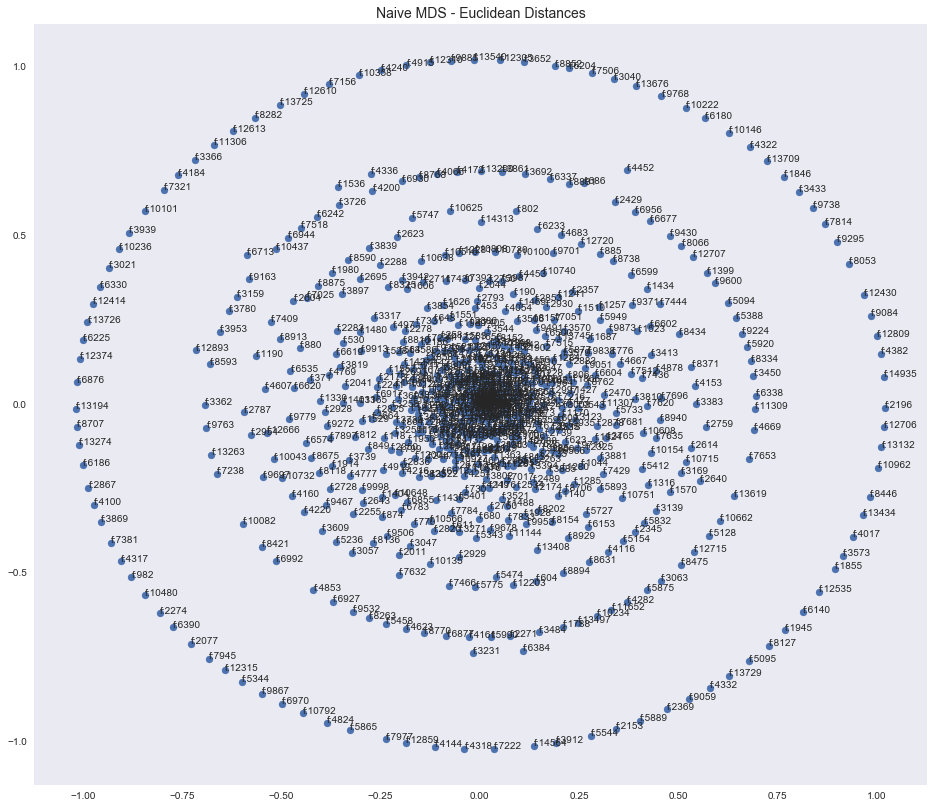
points_euclidean = fit_MDS_2D(euc_dists)
# Create scatter plot of projected points based on Euclidean Distances
simple_scatterplot(points_euclidean[:,0],points_euclidean[:,1],
"Naive MDS - Euclidean Distances",
investors
);
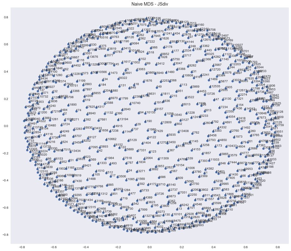
In [24]:
# Fit with MSD
points_JSd = fit_MDS_2D(JSd_dists)

#create scatter plot of projected points based on JSDiv
simple_scatterplot(points_JSd[:,0],points_JSd[:,1],
                   "Naive MDS - JSdiv",
                   investors
                  );
In [25]:
def plot_embedding(data, title='MDS Embedding', savepath=None, palette='viridis',
                   size=7):
    """Plot an MDS embedding dataframe for all presidents.

    Uses Seaborn's `lmplot` to create an x-y scatterplot of the data, encoding the
    value of the investor field into the hue (which can be mapped to any desired
    color palette).

    Parameters
    ----------
    data : DataFrame
        A DataFrame that must contain 3 columns labeled 'x', 'y' and 'investor'.

    title : optional, string
        Title for the plot

    savepath : optional, string
        If given, a path to save the figure into using matplotlib's `savefig`.

    palette : optional, string
        The name of a valid Seaborn palette for coloring the points.

    size : optional, float
        Size of the plot in inches (single number, square plot)

    Returns
    -------
    FacetGrid
        The Seaborn FacetGrid object used to create the plot.
    """
    #process data
    x = data['x']
    y = data['y']
    investor = data['investor']

    #set boolean for using or not using annotation
    do_annotate = False

    #create scatterplot using linear model without a regression fit
    p = sns.lmplot(x = "x", y = "y", data = data, hue = "investor", palette = palette, size = size, fit_reg= False, legend=False)
    p.ax.legend(bbox_to_anchor=(1.01, 0.85),ncol=2)

    #this is used in order to annotate
    ax = plt.gca()

    #make grid and set title
    plt.grid()
    plt.title(title,fontsize=16)

    #adjust border for file saving so not cut-off
    plt.tight_layout()

    #save file
    if (savepath != None):
        plt.savefig(savepath)
In [26]:
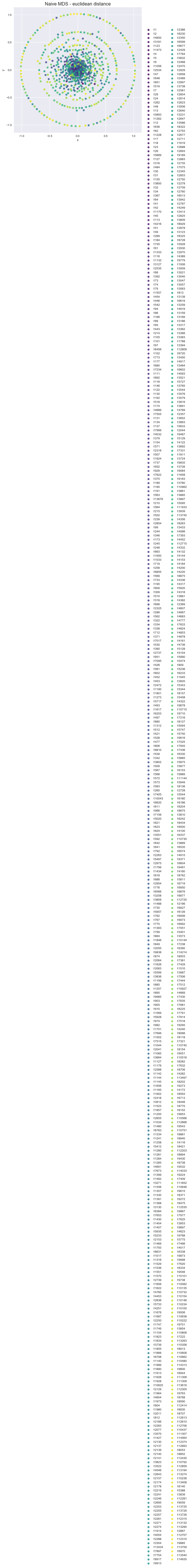
#create embed_peu data frame
embed_peu = pd.DataFrame([])
embed_peu['x'] = points_euclidean[:, 0]
embed_peu['y'] = points_euclidean[:, 1]
embed_peu['investor'] = investors
In [27]:
plot_embedding(embed_peu, 'Naive MDS - euclidean distance', 'results/mds_naive.png');
In [28]:
#create edf2 data frame from JSdiv metric
edf2 = pd.DataFrame([])
edf2['x'] = points_JSd[:, 0]
edf2['y'] = points_JSd[:, 1]
edf2['investor'] = investors
In [29]:
plot_embedding(edf2, 'MDS - Jensen-Shannon Distance', 'results/mds_jsdiv.png');
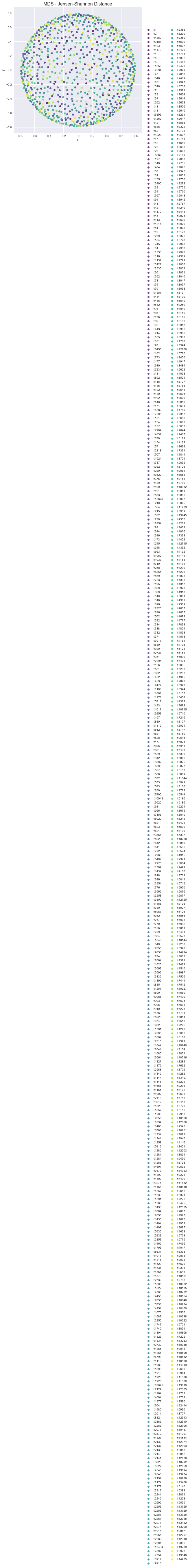
Using this very sparse investor-company distance matrix data we cannot conclude any compelling correlations among investors. We tried a variety of subsets of the data in the hopes that we would discover correlations among investors. For example, some of the attributes that we tried to subset on were:
Top 5% of companies in terms of funding_total_usd
allData = allData.sort_values(by='funding_total_usd', ascending=False)
allData = allData.iloc[0:int(0.05*71811)]
CA
allData = allData[allData.state_code == "CA"]
Biotech
allData = allData[allData.category_code == "biotech"]
However, unfortunately no clusters emerged. Therefore, we condlude that we cannot produce compelling correlations among investors.