Exploratory analyses #1 & #2: the effects of place and time
We begin with exploratory analysis of the various factors we hypothesize may influence a company’s success. In this notebook, we investigate associations between company valuation at IPO or total funding amount and office location and timing.
Set-up
Import stand-alone functions and necessary packages.
In [1]:
from modules import *
In [2]:
%matplotlib inline
import matplotlib.pyplot as plt
import seaborn as sns
import numpy as np
import pandas as pd

plt.style.use('seaborn-dark')
plt.rcParams['figure.figsize'] = (10, 6)
Connect to the MySQL database, read in cb_offices and cb_ipos and convert to dataframes, disconnect from database.
In [3]:
conn = dbConnect()
offices = dbTableToDataFrame(conn, 'cb_offices')
ipos = dbTableToDataFrame(conn, 'cb_ipos')
conn.close()
Look at offices and ipos dataframes & merge them
In [4]:
offices.head()
Out[4]:
| address1 | address2 | city | country_code | created_at | description | id | latitude | longitude | object_id | office_id | region | state_code | updated_at | zip_code | |
|---|---|---|---|---|---|---|---|---|---|---|---|---|---|---|---|
| 0 | 710 - 2nd Avenue | Suite 1100 | Seattle | USA | None | 1 | 47.6031220000 | -122.3332530000 | c:1 | 1 | Seattle | WA | None | 98104 | |
| 1 | 4900 Hopyard Rd | Suite 310 | Pleasanton | USA | None | Headquarters | 2 | 37.6929340000 | -121.9049450000 | c:3 | 3 | SF Bay | CA | None | 94588 |
| 2 | 135 Mississippi St | None | San Francisco | USA | None | None | 3 | 37.7647260000 | -122.3945230000 | c:4 | 4 | SF Bay | CA | None | 94107 |
| 3 | 1601 Willow Road | None | Menlo Park | USA | None | Headquarters | 4 | 37.4160500000 | -122.1518010000 | c:5 | 5 | SF Bay | CA | None | 94025 |
| 4 | Suite 200 | 654 High Street | Palo Alto | ISR | None | 5 | None | None | c:7 | 7 | SF Bay | CA | None | 94301 |
In [5]:
ipos.head()
Out[5]:
| created_at | id | ipo_id | object_id | public_at | raised_amount | raised_currency_code | source_description | source_url | stock_symbol | updated_at | valuation_amount | valuation_currency_code | |
|---|---|---|---|---|---|---|---|---|---|---|---|---|---|
| 0 | 2008-02-09 05:17:45 | 1 | 1 | c:1654 | 1980-12-19 | None | USD | None | None | NASDAQ:AAPL | 2012-04-12 04:02:59 | None | USD |
| 1 | 2008-02-09 05:25:18 | 2 | 2 | c:1242 | 1986-03-13 | None | None | None | None | NASDAQ:MSFT | 2010-12-11 12:39:46 | None | USD |
| 2 | 2008-02-09 05:40:32 | 3 | 3 | c:342 | 1969-06-09 | None | None | None | None | NYSE:DIS | 2010-12-23 08:58:16 | None | USD |
| 3 | 2008-02-10 22:51:24 | 4 | 4 | c:59 | 2004-08-25 | None | None | None | None | NASDAQ:GOOG | 2011-08-01 20:47:08 | None | USD |
| 4 | 2008-02-10 23:28:09 | 5 | 5 | c:317 | 1997-05-01 | None | None | None | None | NASDAQ:AMZN | 2011-08-01 21:11:22 | 100000000000 | USD |
In [6]:
# merge by 'object_id' field, which uniquely links the two dataframes
offices_ipos = pd.merge(offices, ipos, on='object_id')
In [7]:
# look at new merged dataframe
offices_ipos.head()
Out[7]:
| address1 | address2 | city | country_code | created_at_x | description | id_x | latitude | longitude | object_id | ... | ipo_id | public_at | raised_amount | raised_currency_code | source_description | source_url | stock_symbol | updated_at_y | valuation_amount | valuation_currency_code | |
|---|---|---|---|---|---|---|---|---|---|---|---|---|---|---|---|---|---|---|---|---|---|
| 0 | 1601 Willow Road | None | Menlo Park | USA | None | Headquarters | 4 | 37.4160500000 | -122.1518010000 | c:5 | ... | 847 | 2012-05-18 | 18400000000 | USD | Facebook Prices IPO at Record Value | http://online.wsj.com/news/articles/SB10001424... | NASDAQ:FB | 2013-11-21 19:40:55 | 104000000000 | USD |
| 1 | None | None | Dublin | IRL | None | Europe HQ | 6975 | 53.3441040000 | -6.2674940000 | c:5 | ... | 847 | 2012-05-18 | 18400000000 | USD | Facebook Prices IPO at Record Value | http://online.wsj.com/news/articles/SB10001424... | NASDAQ:FB | 2013-11-21 19:40:55 | 104000000000 | USD |
| 2 | 340 Madison Ave | None | New York | USA | None | New York | 9084 | 40.7557162000 | -73.9792469000 | c:5 | ... | 847 | 2012-05-18 | 18400000000 | USD | Facebook Prices IPO at Record Value | http://online.wsj.com/news/articles/SB10001424... | NASDAQ:FB | 2013-11-21 19:40:55 | 104000000000 | USD |
| 3 | 1355 Market St. | None | San Francisco | USA | None | 10 | 37.7768052000 | -122.4169244000 | c:12 | ... | 1310 | 2013-11-07 | 1820000000 | USD | Twitter Prices IPO Above Estimates At $26 Per ... | http://techcrunch.com/2013/11/06/twitter-price... | NYSE:TWTR | 2013-11-07 04:18:48 | 18100000000 | USD | |
| 4 | 2145 Hamilton Avenue | None | San Jose | USA | None | Headquarters | 16 | 37.2950050000 | -121.9300350000 | c:20 | ... | 26 | 1998-10-02 | None | USD | None | None | NASDAQ:EBAY | 2012-04-12 04:24:15 | None | USD |
5 rows × 27 columns
In [8]:
offices_ipos.shape
Out[8]:
(1554, 27)
In [9]:
offices_ipos.columns
Out[9]:
Index(['address1', 'address2', 'city', 'country_code', 'created_at_x',
       'description', 'id_x', 'latitude', 'longitude', 'object_id',
       'office_id', 'region', 'state_code', 'updated_at_x', 'zip_code',
       'created_at_y', 'id_y', 'ipo_id', 'public_at', 'raised_amount',
       'raised_currency_code', 'source_description', 'source_url',
       'stock_symbol', 'updated_at_y', 'valuation_amount',
       'valuation_currency_code'],
      dtype='object')
Distribution of valuation amount
We first want a sense for the total valuation amounts we are considering. The valuations are all < 2x10¹⁰ except for 3 that are >1x10¹¹. While there are 1,554 entries in the merged dataframe, there are only 167 entries that have valuation amount provided. We will continue with analysis of valuation amount but subsequently look at total funding amount instead later in this notebook to increase our sample size.
In [10]:
# plot valuation distribution; include number of companies considering
val = pd.to_numeric(offices_ipos[~offices_ipos.valuation_amount.isnull()].valuation_amount)
a=sns.distplot(val, rug=True);
a.set_title('valuation distribution (N = ' + str(len(val)) + ')');
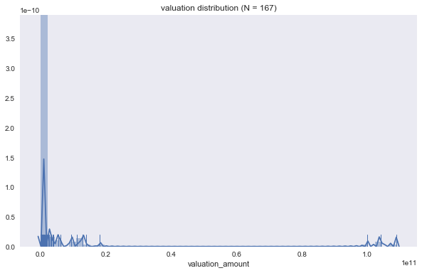
We look at these 3 outliers and see that one is simply because the valuation amount is in JPY (currently 1 JPY = 0.0088 USD). The other two are Facebook and Amazon, which we know to be companies with very high valuations. We will look at those with valuation_currency_code ‘USD’ moving forward to standardize our analysis to one currency.
In [11]:
# look at the 3 outliers with very large valuation_amount
offices_ipos[pd.to_numeric(offices_ipos.valuation_amount) > 0.8e11]
Out[11]:
| address1 | address2 | city | country_code | created_at_x | description | id_x | latitude | longitude | object_id | ... | ipo_id | public_at | raised_amount | raised_currency_code | source_description | source_url | stock_symbol | updated_at_y | valuation_amount | valuation_currency_code | |
|---|---|---|---|---|---|---|---|---|---|---|---|---|---|---|---|---|---|---|---|---|---|
| 0 | 1601 Willow Road | None | Menlo Park | USA | None | Headquarters | 4 | 37.4160500000 | -122.1518010000 | c:5 | ... | 847 | 2012-05-18 | 18400000000 | USD | Facebook Prices IPO at Record Value | http://online.wsj.com/news/articles/SB10001424... | NASDAQ:FB | 2013-11-21 19:40:55 | 104000000000 | USD |
| 1 | None | None | Dublin | IRL | None | Europe HQ | 6975 | 53.3441040000 | -6.2674940000 | c:5 | ... | 847 | 2012-05-18 | 18400000000 | USD | Facebook Prices IPO at Record Value | http://online.wsj.com/news/articles/SB10001424... | NASDAQ:FB | 2013-11-21 19:40:55 | 104000000000 | USD |
| 2 | 340 Madison Ave | None | New York | USA | None | New York | 9084 | 40.7557162000 | -73.9792469000 | c:5 | ... | 847 | 2012-05-18 | 18400000000 | USD | Facebook Prices IPO at Record Value | http://online.wsj.com/news/articles/SB10001424... | NASDAQ:FB | 2013-11-21 19:40:55 | 104000000000 | USD |
| 91 | 1200 12th Ave | S # 1200 | Seattle | USA | None | None | 288 | 47.5923000000 | -122.3172950000 | c:317 | ... | 5 | 1997-05-01 | None | None | None | None | NASDAQ:AMZN | 2011-08-01 21:11:22 | 100000000000 | USD |
| 360 | Roppongi-Hills Mori Tower, 6-10-1, Roppongi | Minato-ku | Tokyo | JPN | None | Headquarters | 9085 | None | None | c:15609 | ... | 78 | 2008-12-17 | None | None | None | None | 3632 | 2010-10-08 06:47:07 | 108960000000 | JPY |
5 rows × 27 columns
The above table reveals that we do have duplicate entries for certain companies based on multiple office locations. We need to look at the number of unique companies we are considering, which as shown below is 101 (not 167). Because the ‘description field’ does not sufficiently and uniformly describe the type of office for all entries, we will not filter by that column. Instead, this is just a preliminary exploratory analysis that will keep all locations in the analysis. We would ideally like to filter by ‘Headquarters’ or ‘HQ’ but the data is not sufficiently documented so this would require substantial data entry to designate the headquarters location for all companies with multiple office locations.
In [12]:
len(pd.unique(offices_ipos[~offices_ipos.valuation_amount.isnull()].object_id))
Out[12]:
101
Valuation amount by region
We want to determine the effect of location on IPO valuation. In particular, we consider the median valuation and number of IPOs by region to determine whether certain regions are hotspots for companies that IPO. As mentioned above, we now limit our analysis to valuations in USD, which reduces our N from 167 to 161.
In [13]:
# restrict to valuations in USD currency
offices_ipos_us = offices_ipos[offices_ipos.valuation_currency_code == 'USD']
val_us = pd.to_numeric(offices_ipos_us[~offices_ipos_us.valuation_amount.isnull()].valuation_amount)
region = offices_ipos_us[~offices_ipos_us.valuation_amount.isnull()].region
# create dataframe with just region and valuation
df_region_val = pd.concat([region, val_us], axis=1)
df_region_val.describe()
Out[13]:
| valuation_amount | |
|---|---|
| count | 1.610000e+02 |
| mean | 3.904637e+09 |
| std | 1.615982e+10 |
| min | 3.860000e+04 |
| 25% | 1.340000e+08 |
| 50% | 3.150000e+08 |
| 75% | 1.000000e+09 |
| max | 1.040000e+11 |
In [14]:
# perform calculations on a per region basis
reg = df_region_val.groupby(['region'])
SF Bay has the most IPOs with NY, London, and Seattle following.
In [15]:
# sort regions by number of ipos (that had valutation amount listed)
num = reg.count()
num.sort_values(by='valuation_amount', ascending=False)[0:10]
Out[15]:
| valuation_amount | |
|---|---|
| region | |
| SF Bay | 34 |
| New York | 11 |
| London | 8 |
| Seattle | 7 |
| Denver | 6 |
| Boston | 6 |
| Los Angeles | 6 |
| Chicago | 5 |
| Beijing | 4 |
| Singapore | 3 |
To create an informative boxplot of valuation amount by region we include regions with >5 companies that IPO.
In [16]:
# plot valuation by region
top7 = ['SF Bay', 'New York', 'London', 'Seattle', 'Denver', 'Boston', 'Los Angeles']
df_top7 = df_region_val[df_region_val.region.isin(top7)]
fig, a = plt.subplots(figsize=(16,10))
a=sns.barplot(x='region', y='valuation_amount',data=df_top7, ci=False, order=top7)
a.set_ylabel('valuation amount')
a.set_title('valuation by region')
plt.xticks(rotation=90);
plt.savefig('results/valuation_region.png')
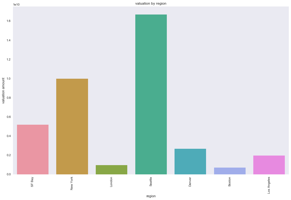
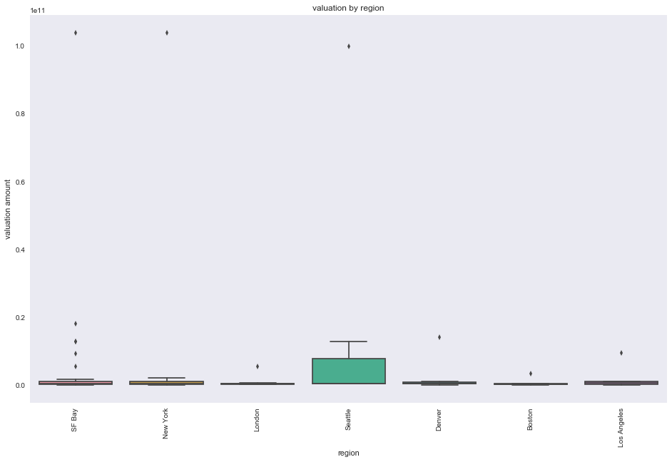
While SF Bay has the most companies that IPO (above barplot is sorted from most companies that IPO to least), the region with the highest mean valuation amount is Seattle. However, the N for Seattle is only 7 so the effects of outliers like Microsoft are more significant (refer to wider boxplot for Seattle below).
In [17]:
# plot valuation by region
top7 = ['SF Bay', 'New York', 'London', 'Seattle', 'Denver', 'Boston', 'Los Angeles']
df_top7 = df_region_val[df_region_val.region.isin(top7)]
fig, a = plt.subplots(figsize=(16,10))
a=sns.boxplot(x='region', y='valuation_amount',data=df_top7, order=top7)
a.set_ylabel('valuation amount')
a.set_title('valuation by region')
plt.xticks(rotation=90);
Analysis of number of IPOs over time
In addition to looking at the value and region of companies that IPO we also look at historical trends in terms of the number of IPOs over time to determine how timing may affect a company’s success. We no longer restrict analysis to companies where valuation amount is provided.
In [18]:
# now don't filter to ones with valuation amount only
dt = pd.to_datetime(offices_ipos.public_at)
valAll = pd.to_numeric(offices_ipos.valuation_amount)
regionAll = offices_ipos.region
In [19]:
df_region_dt = pd.concat([regionAll, dt], axis=1)
time = df_region_dt.groupby([dt.dt.year])
In [20]:
# top counts by year
num = time.count()
num.sort_values(by='public_at', ascending=False).head(10)
Out[20]:
| region | public_at | |
|---|---|---|
| public_at | ||
| 2013.0 | 154 | 154 |
| 2004.0 | 88 | 88 |
| 2011.0 | 83 | 83 |
| 2010.0 | 77 | 77 |
| 2012.0 | 51 | 51 |
| 2009.0 | 47 | 47 |
| 1999.0 | 47 | 47 |
| 2007.0 | 46 | 46 |
| 2008.0 | 44 | 44 |
| 2000.0 | 43 | 43 |
In [21]:
# barplot showing number of ipos by year
a=sns.barplot(num.public_at.index, num.public_at)
a.set_ylabel('number of ipos')
a.set_xlabel('year')
a.set_title('number of ipos by year');
a.set_xticklabels(labels=num.public_at.index.astype(int), rotation=90);
plt.savefig('results/ipos_year.png')
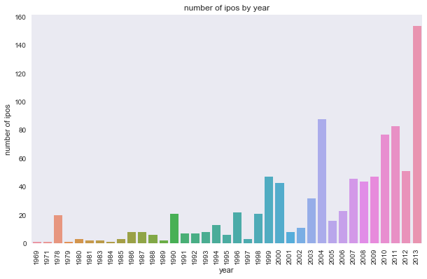
More recent years have more IPOs. However, we cannot rule out the possibility that the Crunchbase dataset is also simply becoming more complete.
Incorporate cb_objects into analysis to consider funding_total_usd metric
While we had been considering valuation amount from the IPO data, we also consider funding_total_usd for the below analysis because it is a much richer dataset. We have N=27,874 instead of N=167.
Connect to database and look at dataframe from cb_objects
In [22]:
conn = dbConnect()
objs = dbTableToDataFrame(conn, 'cb_objects')
conn.close()
In [23]:
objs.head()
Out[23]:
| category_code | city | closed_at | country_code | created_at | created_by | description | domain | entity_id | entity_type | ... | parent_id | permalink | region | relationships | short_description | state_code | status | tag_list | twitter_username | updated_at | |
|---|---|---|---|---|---|---|---|---|---|---|---|---|---|---|---|---|---|---|---|---|---|
| 0 | web | Seattle | None | USA | 2007-05-25 06:51:27 | initial-importer | Technology Platform Company | wetpaint-inc.com | 1 | Company | ... | None | /company/wetpaint | Seattle | 17.0 | None | WA | operating | wiki, seattle, elowitz, media-industry, media-... | BachelrWetpaint | 2013-04-13 03:29:00 |
| 1 | games_video | Culver City | None | USA | 2007-05-31 21:11:51 | initial-importer | None | flektor.com | 10 | Company | ... | None | /company/flektor | Los Angeles | 6.0 | None | CA | acquired | flektor, photo, video | None | 2008-05-23 23:23:14 |
| 2 | games_video | San Mateo | None | USA | 2007-08-06 23:52:45 | initial-importer | there.com | 100 | Company | ... | None | /company/there | SF Bay | 12.0 | None | CA | acquired | virtualworld, there, teens | None | 2013-11-04 02:09:48 | |
| 3 | network_hosting | None | None | None | 2008-08-24 16:51:57 | None | None | mywebbo.com | 10000 | Company | ... | None | /company/mywebbo | unknown | NaN | None | None | operating | social-network, new, website, web, friends, ch... | None | 2008-09-06 14:19:18 |
| 4 | games_video | None | None | None | 2008-08-24 17:10:34 | None | None | themoviestreamer.com | 10001 | Company | ... | None | /company/the-movie-streamer | unknown | NaN | None | None | operating | watch, full-length, moives, online, for, free,... | None | 2008-09-06 14:19:18 |
5 rows × 40 columns
In [24]:
objs.columns
Out[24]:
Index(['category_code', 'city', 'closed_at', 'country_code', 'created_at',
       'created_by', 'description', 'domain', 'entity_id', 'entity_type',
       'first_funding_at', 'first_investment_at', 'first_milestone_at',
       'founded_at', 'funding_rounds', 'funding_total_usd', 'homepage_url',
       'id', 'invested_companies', 'investment_rounds', 'last_funding_at',
       'last_investment_at', 'last_milestone_at', 'logo_height', 'logo_url',
       'logo_width', 'milestones', 'name', 'normalized_name', 'overview',
       'parent_id', 'permalink', 'region', 'relationships',
       'short_description', 'state_code', 'status', 'tag_list',
       'twitter_username', 'updated_at'],
      dtype='object')
In [25]:
objs.shape
Out[25]:
(462651, 40)
In [26]:
len(objs.funding_total_usd[~objs.funding_total_usd.isnull()])
Out[26]:
27874
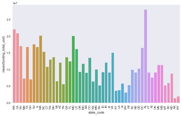
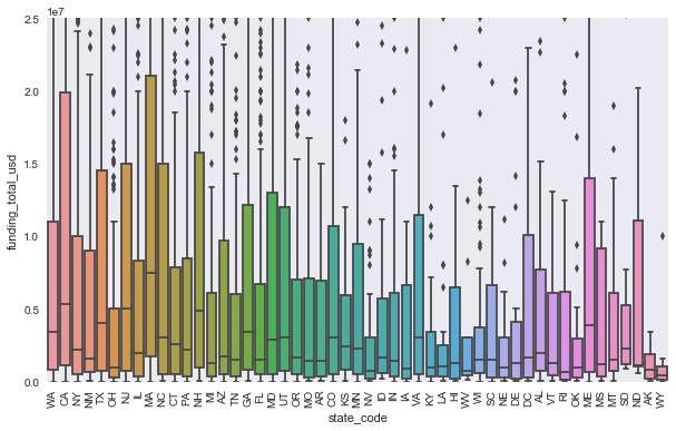
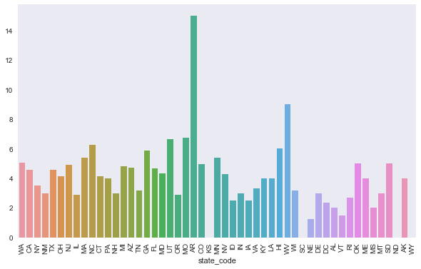
Look at the influence of state on total funding
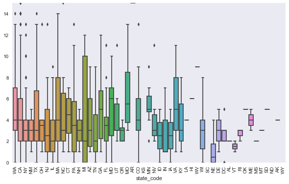
The greatest mean funding is in WA, CA, MA, MD, and AL. However when looking at boxplots with the median indicated, which is a better metric so we are not sensitive to extreme outliers, we see that the median is highest in CA, MA, NJ, NH, and ME.
In [27]:
# plot mean funding_total_usd by state
a=sns.barplot(objs['state_code'], pd.to_numeric(objs['funding_total_usd']), ci=False);
plt.xticks(rotation=90);
In [28]:
# boxplot of funding_total_usd by state
a=sns.boxplot(objs['state_code'], pd.to_numeric(objs['funding_total_usd']));
a.set_ylim(0, 2.5e7)
plt.xticks(rotation=90);
plt.savefig('results/funding_state.png')
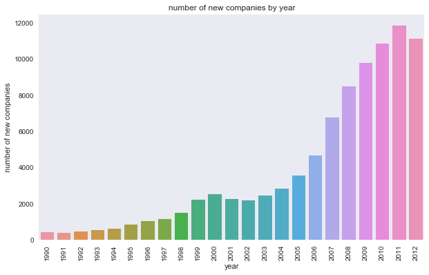
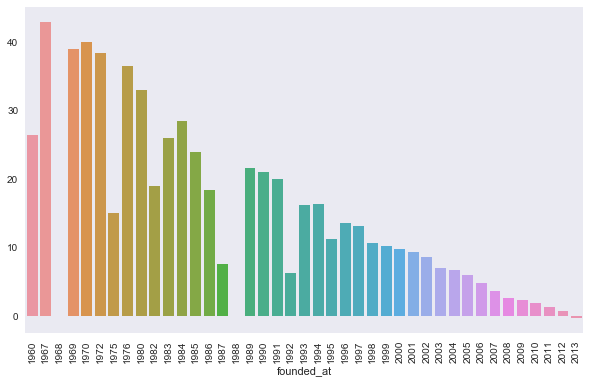
Just as we looked at the number of IPOs over time, we now look at the emergence of new companies over time.
In [29]:
# group by date founded to do analysis on the emergence of new companies over time
dt = pd.to_datetime(objs.founded_at)
df_fund_dt = pd.concat([objs.funding_total_usd, dt], axis=1)
founded = df_fund_dt.groupby([dt.dt.year])
In [30]:
# top counts by year
num_found = founded.count()
num_found.sort_values(by='founded_at', ascending=False)['founded_at'].head(10)
Out[30]:
founded_at
2011.0    11884
2012.0    11158
2010.0    10858
2009.0     9805
2008.0     8502
2007.0     6765
2013.0     6280
2006.0     4689
2005.0     3580
2004.0     2828
Name: founded_at, dtype: int64
In [31]:
# plot number of new companies by year; zooming in on 1990 and later where there is more data
a=sns.barplot(num_found.founded_at.index.astype(int)[(num_found.founded_at.index.astype(int) >= 1990)
                                                     & (num_found.founded_at.index.astype(int) < 2013)],
              num_found.founded_at[(num_found.founded_at.index.astype(int) >= 1990)
                                   & (num_found.founded_at.index.astype(int) < 2013)])
a.set_ylabel('number of new companies')
a.set_xlabel('year')
a.set_title('number of new companies by year');
plt.xticks(rotation=90);
plt.savefig('results/new_year.png')
In [32]:
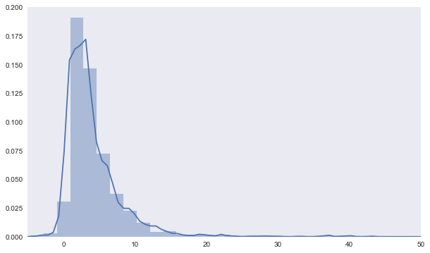
# company lifespan: closed_at - founded_at
start = pd.to_datetime(objs.founded_at)
end = pd.to_datetime(objs.closed_at)
life = end.dt.year - start.dt.year
In [33]:
a=sns.distplot(life[~life.isnull()]);
a.set_xlim(-5, 50);
In [34]:
# there are 27 with a life < 0 showing data entry for this data set was flawed.
life[life < 0].describe()
Out[34]:
count    27.000000
mean     -7.851852
std      10.614590
min     -40.000000
25%      -9.500000
50%      -3.000000
75%      -1.000000
max      -1.000000
dtype: float64
In [35]:
# consider those with positive life
life_pos = life[life>0]
life_pos[~life_pos.isnull()].describe()
Out[35]:
count    2013.000000
mean        4.384004
std         4.359592
min         1.000000
25%         2.000000
50%         3.000000
75%         5.000000
max        53.000000
dtype: float64
In [36]:
# see whether companies tend to have longer of shorter lifespans based on when they were founded
a=sns.barplot(start[~life.isnull()].dt.year.astype(int), life[~life.isnull()], ci=None);
plt.xticks(rotation=90);
In [37]:
# see whether companies tend to have longer or shorter lifespans based on region
a=sns.barplot(objs.state_code[~objs.state_code.isnull()], life[~objs.state_code.isnull()], ci=None);
plt.xticks(rotation=90);
In [38]:
# see whether companies tend to have longer or shorter lifespans based on region
a=sns.boxplot(objs.state_code[~objs.state_code.isnull()], life[~objs.state_code.isnull()]);
a.set_ylim(0,15);
plt.xticks(rotation=90);