Exploratory Analysis #4: Executive Education

So you want to start a company…

The leaders of the world’s top businesses have to start somewhere. Using the Crunchbase data, we take a look at where these business leaders received their educations. Is it true that you need to attend a world class institution to be successful, or is the business world much more varied in terms of educational backgrounds?

% matplotlib inline
# Overhead
import MySQLdb
import seaborn as sns
import pandas as pd
import numpy as np
from matplotlib import pyplot as plt
from IPython.display import display
from modules import *

Since the crunchbase data is in the form of MySQL database dumps, we have already loaded this information into a MySQL database locally. See ___________ for instructions if you have not done this already.

Next, we connect to that database and save a couple information tables locally as pandas DataFrames.

conn = dbConnect()
people = dbTableToDataFrame(conn,'cb_people')
degrees = dbTableToDataFrame(conn,'cb_degrees')
funding_rounds = dbTableToDataFrame(conn,'cb_funding_rounds')
objects = dbTableToDataFrame(conn,'cb_objects')
conn.close()

Username: root
Password: ········

The most successful businesses

If we consider a successful business to be one that has raised the most capital through a variety of funding rounds, we can sort our dataset accordingly.

We can get the total raised by a company by using the funding_total_usd column in the objects database. Note that we only want to use companies, so we only select those with an entity_type of “company”. We will also reduce the size of our dataframe to include only a couple important metrics.

companies = objects[objects.entity_type=='Company'][['name','entity_id','funding_total_usd','closed_at']].copy()
# Only select companies who have raised some money
companies = companies.dropna(subset=['funding_total_usd'])
display(companies.sort_values('funding_total_usd',ascending=False).head(10))

comp_tot = len(companies)
print('There are {:,} companies in the dataset'.format(comp_tot))

	name	entity_id	funding_total_usd	closed_at
4575	Clearwire	13219	5700000000	None
160023	Verizon Communications, Inc.	4843	3985050000	None
97784	sigmacare	242735	2600000000	None
161551	Facebook	5	2425700000	None
175825	Carestream	64365	2400000000	None
81001	Solyndra	22568	1765504319	None
170979	Fisker Automotive	5951	1451000000	None
151715	O3b Networks	39799	1270283000	None
101987	Terra-Gen Power	24693	1200000000	None
2971	Twitter	12	1160166511	None

There are 27,874 companies in the dataset

Now that we have all of the companies, let’s define exactly what we mean by the most successful companies. First, to get a feel for the data visually, let’s look at the top 100 companies and their fundraising totals.

fig,ax = plt.subplots(figsize=(20,20))
n_top_companies = 100
plotset = companies.sort_values('funding_total_usd',ascending=False).head(n_top_companies)
ax = sns.barplot(x='funding_total_usd',y='name',data=plotset)
ax.set_title('Funding Totals for the Top {} Companies'.format(n_top_companies),fontsize=22)
ax.set_xscale('log')
ax.set_xlabel('Funding Total [USD] -- Log Scale',fontsize=18);
ax.set_yticklabels(labels=plotset.name)
ax.set_ylabel('Company',fontsize=18)
plt.savefig('results/funding_totals.png')

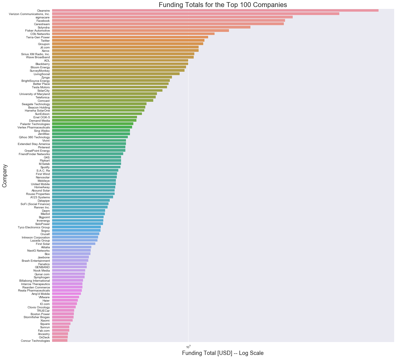
Note that the y-axis is on a logarithmic scale, and so the visible trend is dramatically underexaggerated.

It appears that only a handful of the companies fundraise greater than $1 billion ($:math:10^9), though many more companies appear to fundraise in the millions. Let’s find the exact percent of companies for each order of magnitude.

I,F = 3,10
for i in np.logspace(I,F,F-I+1):
    num_above = len(companies[companies['funding_total_usd']>i])
    frac = num_above/comp_tot
    print('{:,} companies ({}%) above ${:,}'.format(num_above,round(100*frac,1),int(i)))

27,854 companies (99.9%) above $1,000
27,608 companies (99.0%) above $10,000
24,960 companies (89.5%) above $100,000
18,112 companies (65.0%) above $1,000,000
7,309 companies (26.2%) above $10,000,000
630 companies (2.3%) above $100,000,000
15 companies (0.1%) above $1,000,000,000
0 companies (0.0%) above $10,000,000,000

We see from this that only slightly more than 25% of the companies fundraise more than $10 million. Let’s define these 7309 companies as the most successful.

The people behind the most successful businesses

Next, we can use the people database to pair individuals with the company they are affiliated with. Like for the funding rounds data, we don’t need all of the information provided in the database of people either. Since we ultimately want to look at educational factors, let’s limit the dataset to only a person’s name (first and last), object_id, and affiliation, in a key that will let us link to the degrees dataset.

people_key = people[['affiliation_name','first_name','last_name','object_id']]
display(people_key.head(10))

ppl_tot = len(people_key)
print('There are {:,} people in the dataset'.format(ppl_tot))

	affiliation_name	first_name	last_name	object_id
0	Blue Nile	Ben	Elowitz	p:2
1	Wetpaint	Kevin	Flaherty	p:3
2	Zoho	Raju	Vegesna	p:4
3	Zoho	Ian	Wenig	p:5
4	i/o Ventures	Kevin	Rose	p:6
5	Digg	Jay	Adelson	p:7
6	Digg	Owen	Byrne	p:8
7	Digg	Ron	Gorodetzky	p:9
8	Facebook	Mark	Zuckerberg	p:10
9	Facebook	Dustin	Moskovitz	p:11

There are 226,709 people in the dataset

Now we merge the two datasets together to get each funded company and people in the crunchbase dataset who were involved.

company_people = pd.merge(companies,people_key,left_on='name',right_on='affiliation_name').drop('affiliation_name',axis=1)
display(company_people.head())

cp_tot = len(company_people)
print('There are {:,} people affiliated with funded companies in the dataset'.format(cp_tot))

	name	entity_id	funding_total_usd	closed_at	first_name	last_name	object_id
0	Wetpaint	1	39750000	None	Kevin	Flaherty	p:3
1	Wetpaint	1	39750000	None	Alex	Weinstein	p:104800
2	FriendFeed	1001	5000000	None	Paul	Buchheit	p:640
3	FriendFeed	1001	5000000	None	Sanjeev	Singh	p:2716
4	Fitbit	10015	68069200	None	James	Park	p:16930

There are 12,168 people affiliated with funded companies in the dataset

Interestingly, there are significantly fewer people associated with companies than there are people in the dataset.

We can now repeat the merging process with the dataset of educational information. First, let’s limit the degrees dataset to include only degree type, institution, subject, and the id of the corresponding person (object_id). Then, we merge this into the database of companies and people.

edu = degrees[['object_id','institution','degree_type','subject']].dropna(subset=['institution'])
CPE = pd.merge(company_people,edu,on='object_id')
display(CPE.head(10))

	name	entity_id	funding_total_usd	closed_at	first_name	last_name	object_id	institution	degree_type	subject
0	Wetpaint	1	39750000	None	Kevin	Flaherty	p:3	Washington University in St Louis	BBA	None
1	Wetpaint	1	39750000	None	Kevin	Flaherty	p:3	Indiana University	MBA	None
2	FriendFeed	1001	5000000	None	Paul	Buchheit	p:640	Case Western Reserve University	MS	Computer Science
3	FriendFeed	1001	5000000	None	Sanjeev	Singh	p:2716	Stanford University	BS	Computer Science
4	Fitbit	10015	68069200	None	James	Park	p:16930	Harvard University	DNF	Computer Science
5	Fitbit	10015	68069200	None	Eric	Friedman	p:16931	George Washington University	BBA	Business Marketing
6	Fitbit	10015	68069200	None	Meena	Srinivasan	p:89236	India, Certified Public Accountant in California	Chartered Accountant	None
7	Fitbit	10015	68069200	None	Meena	Srinivasan	p:89236	East Carolina University	MBA	None
8	Fitbit	10015	68069200	None	Mark	Silverio	p:121130	Boston College	BS	Marketing
9	Fitbit	10015	68069200	None	Eric	Friedman	p:216979	Yale University	MS	Computer Science

Finally, we filter the dataset of company, people, and education to only those in the most successful businesses (those who fundraised more than $10 million).

successful_CPE = CPE[CPE['funding_total_usd']>10_000]
display(successful_CPE.head())

n_entries = len(CPE)
n_unique_ppl = CPE['object_id'].nunique()
print('There are {:,} entries in the dataset, and {:,} unique people in the dataset.'.format(n_entries,n_unique_ppl))
print('On average, successful businesses involve people with an average of {} degrees.'.format(round(n_entries/n_unique_ppl,1)))

	name	entity_id	funding_total_usd	closed_at	first_name	last_name	object_id	institution	degree_type	subject
0	Wetpaint	1	39750000	None	Kevin	Flaherty	p:3	Washington University in St Louis	BBA	None
1	Wetpaint	1	39750000	None	Kevin	Flaherty	p:3	Indiana University	MBA	None
2	FriendFeed	1001	5000000	None	Paul	Buchheit	p:640	Case Western Reserve University	MS	Computer Science
3	FriendFeed	1001	5000000	None	Sanjeev	Singh	p:2716	Stanford University	BS	Computer Science
4	Fitbit	10015	68069200	None	James	Park	p:16930	Harvard University	DNF	Computer Science

There are 10,823 entries in the dataset, and 6,768 unique people in the dataset.
On average, successful businesses involve people with an average of 1.6 degrees.

We see that out of the 12,168 people in the full dataset, more than half are associated with well performing businesses. We also see that it is quite common for those at successful businesses to have multiple degrees.

(Not so) humble beginnings

Next we take a look at the institutions who have produced the people affiliated with the successful businesses. If we were to take a closer look at the table above, you would see that many of the institutions are duplicated, but often with slight variations for each school.

We will try to eliminate some of these duplicates, while at the same time reducing the names in such a way that we can properly aggregate a school when it is named alternatively. We will do this by defining a function which processes a list of school names, removes punctuation and superfluous word (often we are not interested in specific business schools or law schools, and we want inputs like “University of California–Berkeley” and “University of California, Berkeley” to be treated the same. Note: the function defined here relies on a more complicated “SchoolTools” class which is contained in the modules module.

def identify_institutions(institutions):
    '''
    Identify institutions using a common name.

    Each person in the database has a university which was input by a user.
    These inputs are not uniform, and so names are inconsistent for some schools.
    (e.g. Berkeley could be UC Berkeley, Cal, or The University of California)

    Parameters
    ----------
    institutions : Series
        A series giving a list of institutions to be identified.

    Returns
    -------
    inst : Series
        A series where insitutions have been commonly identified.

    '''
    ST = SchoolTools()
    # Make all words lowercase
    inst=institutions.str.lower()
    #Remove stopwords
    inst = ST.remove_stopwords(inst)
    # Remove punctuation
    inst = ST.remove_punctuation(inst)
    # Replace common stems with just the stem, delete others, and replace keywords and nicknames with a common title.
    inst = ST.identify_schools(inst)
    return inst.str.title()

cpe = CPE.copy()
cpe.institution=identify_institutions(cpe.institution)

This dataset is still quite large by itself. To reduce it’s size, we will only focus on those schools which have contributed 15 or more people to successful businesses.

people_contributed_min = 15
inst_counts = pd.DataFrame(cpe.institution.value_counts())
inst_counts = inst_counts.rename(columns={'institution':'total'})
inst_mult = inst_counts[inst_counts.total>=people_contributed_min]
cpe_count = pd.merge(cpe,inst_mult,left_on='institution',right_index=True).sort_values('total',ascending=False)
cpe_count.head()

	name	entity_id	funding_total_usd	closed_at	first_name	last_name	object_id	institution	degree_type	subject	total
10708	Zillow	959	96627980	None	Christopher	Roberts	p:2556	Stanford	BS	Mechanical Engineering	618
7501	Facebook	5	2425700000	None	Sandra Liu	Huang	p:15296	Stanford	BS	Computer Science	618
6930	Apture	4421	4600000	None	Can	Sar	p:18982	Stanford	BS	Computer Science	618
6931	Apture	4421	4600000	None	Can	Sar	p:18982	Stanford	MS	Computer Science	618
7040	MUBI	4524	8245630	None	Efe	Cakarel	p:9537	Stanford	MBA	None	618

To make more sense of this dataset, we will plot according to universities which have contributed the most people to successful businesses.

fig,edu_ax = plt.subplots(figsize=(16,25))
fig.suptitle('Graduates contributed to the most successful businesses by college',fontsize=22,x=0.55,y=1.01)

edu_ax = sns.barplot(x='total',y='institution',data=cpe_count)
edu_ax.tick_params(labelsize=18)
edu_ax.xaxis.tick_top()
edu_ax.set_xlabel('Number of graduates',fontsize=18);
edu_ax.xaxis.set_label_position('top')
edu_ax.set_yticklabels(labels=cpe_count.institution.unique(),fontsize=12)
edu_ax.set_ylabel('School',fontsize=18)

fig.tight_layout()
plt.savefig('results/affiliates_by_school.png')

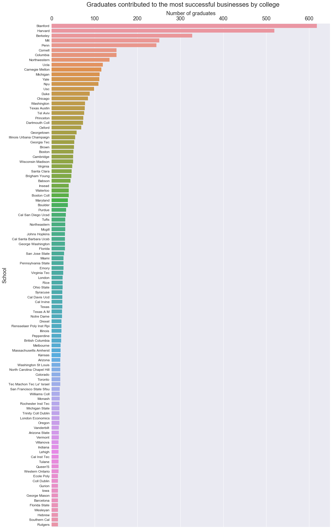
We can see that there are several universities contributing far more graduates to the top businesses than the rest. Just the top three schools (Stanford, Harvard, and UC Berkeley) produce more than 13% of executives and founders of these companies.

cum_frac = 0
for top_school in ['Stanford','Harvard','Berkeley']:
    frac = inst_counts.total.loc[top_school]/inst_counts.total.sum()
    cum_frac += frac
    print('{} has {}% of the total graduates in top businesses.'.format(top_school,round(100*frac,1)))
print('Together, these three schools produced {}% of the total graduates in top businesses.'.format(round(100*cum_frac,1)))

Stanford has 5.7% of the total graduates in top businesses.
Harvard has 4.8% of the total graduates in top businesses.
Berkeley has 3.0% of the total graduates in top businesses.
Together, these three schools produced 13.5% of the total graduates in top businesses.